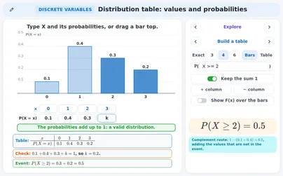
A random variableX gives every outcome of an experiment a number. Its distribution table lists each value x with its probability P(X=x).
Example
Two fair coins, X = the number of heads. HH, HT, TH, TT are equally likely.P(X=0)=41, P(X=1)=42=21, P(X=2)=41.
Rule
The probabilities add up to 1
Every probability is between 0 and 1, and together they make exactly 1 → ∑P(X=x)=1. A table that does not add up to 1 is not a distribution.
Example
0.1+0.4+0.3+0.2=1 → a valid table.0.2+0.5+0.4=1.1 → not valid, whatever the values of X are.
Rule
Find k
When a probability is unknown or holds k, put the sum equal to 1 and solve for k. If k is squared there are two roots: reject the one that gives a negative probability or one above 1.
Example
P(X=x)=kx for x=1,2,3,4.k+2k+3k+4k=10k=1, so k=0.1 and the table is 0.1,0.2,0.3,0.4.
Rule
P(X ≥ a) and the complement
The probability of an event is the sum of the probabilities of the values in it. Often the complement is shorter → P(X≥a)=1−P(X<a).
Example
x=1,2,3,4,5 with P=0.05,0.1,0.15,0.3,0.4.P(X≥2)=1−P(X=1)=1−0.05=0.95, the same as 0.1+0.15+0.3+0.4.
Definition
A table by counting a machine
When dice, coins or a spinner make X, list the equally likely outcomes and count the ways to get each value; P(X=x) is the number of ways divided by the number of outcomes.
Example
Two dice, X = the sum. 7 is made in 6 of the 36 pairs.P(X=7)=366=61.
Tip
Relative frequencies against the theory
An experiment gives counts. Divide each count by the total to get relative frequencies and compare them with the theoretical probabilities: they are close, not equal, and come closer with more repeats.
Example
A spinner with P=0.5,0.3,0.2 is spun 200 times → 96,63,41.Relative frequencies 0.48,0.315,0.205; the largest gap to the theory is 0.02.
Definition
F(x) and P(a < X ≤ b)
F(x)=P(X≤x) adds the probabilities up to and including x. Its graph is a staircase that never goes down and ends at 1. P(a<X≤b)=F(b)−F(a).
Example
x=0,1,2,3 with P=0.1,0.4,0.3,0.2 gives F=0.1,0.5,0.8,1.P(0<X≤2)=F(2)−F(0)=0.8−0.1=0.7.
Definition
E(X) as a weighted mean
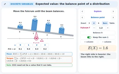
The expected valueE(X)=μ is the mean of the distribution: multiply each value by its probability and add, E(X)=∑xP(X=x).
Example
x=0,1,2,3 with P=0.1,0.4,0.3,0.2.E(X)=0⋅0.1+1⋅0.4+2⋅0.3+3⋅0.2=1.6. The plain mean 1.5 of the four values ignores the weights.
Definition
E(X) as a balance point
Put the bars on a beam as weights. It balances at μ, where the pulls (x−μ)P(X=x) on the two sides cancel. A fulcrum anywhere else tilts the beam to the heavier side.
Example
Fulcrum at 2 for the table above → ∑(x−2)P(X=x)=−0.2−0.4+0+0.2=−0.4.Negative, so the beam tilts left. At 1.6 the sum is 0.
Special case
E(X) need not be a value of X
A fair die has E(X)=3.5, a number no throw gives. E(X) is the long-run average, not the most likely value, and it always lies between the smallest and the largest value.
Example
X=0 or 1, each with P=0.5.E(X)=0⋅0.5+1⋅0.5=0.5, a value X can never take.
Rule
The long run
The mean of many repeats settles near E(X). The typical gap for n repeats is about σ/n, and 2σ/n covers most runs: four times as many repeats halve the gap.
Example
A die thrown by the computer (a fixed seed): the mean of the first 10 is 2.90, of 100 is 3.33, of 1000 is 3.548.Each is within 2σ/n=1.08,0.34,0.11 of 3.5.
Definition
Var(X): the average squared distance
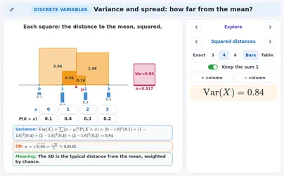
The varianceVar(X)=E((X−μ)2)=∑(x−μ)2P(X=x) is the average of the squared distances to the mean. Squares make every distance count and big distances count most.
Example
μ=1.6: the squared distances for x=0,1,2,3 are 2.56,0.36,0.16,1.96.Var=2.56⋅0.1+0.36⋅0.4+0.16⋅0.3+1.96⋅0.2=0.84.
Rule
A shortcut: E(X²) − μ²
Var(X)=E(X2)−μ2: the mean of the squares minus the square of the mean. It needs no distances and gives the same number, never a negative one.
Example
A fair die → E(X2)=61+4+9+16+25+36=691 and μ2=449.Var=12182−12147=1235.
Definition
Standard deviation and its unit
The standard deviationσ=Var(X) is a typical distance from the mean, in the unit of X. The variance is in the unit squared: minutes give minutes².
Example
Minutes late → 0,5,10 with P=0.5,0.3,0.2.E(X)=3.5, E(X2)=27.5, Var=27.5−3.52=15.25 min², σ=15.25≈3.91 min.
Watch out!
Same mean, different spread
Two distributions can have the same E(X) and still be very different: the mean says where the middle is, the standard deviation says how far the values lie from it. Give both.
Example
A → 1,2,3 and B → 0,2,4, both with P=0.25,0.5,0.25.Both have E=2, but Var(A)=0.5 and Var(B)=2, so σB=2 is twice σA=22.
Rule
The new variable aX + b
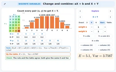
For Y=aX+b → E(Y)=aE(X)+b and Var(Y)=a2Var(X), so σY=∣a∣σX. Adding b moves the table, multiplying by a stretches it.
Example
X → 0,1,2,3 with P=0.1,0.4,0.3,0.2 (E=1.6, Var=0.84). Y=3X−2.E(Y)=3⋅1.6−2=2.8, Var(Y)=32⋅0.84=7.56, σY=3σX≈2.75.
Watch out!
b never counts, a is squared
b never changes the spread. A variance is never negative, so a is squared → Var(−X)=Var(X), not −Var(X). The standard deviation uses ∣a∣.
Example
X as above, Y=10−2X.E(Y)=10−2⋅1.6=6.8, Var(Y)=(−2)2⋅0.84=3.36 (not −3.36), σY=2σX≈1.83.
Rule
X + Y: the independence rule
E(X+Y)=E(X)+E(Y) always. For independentX and Y also Var(X+Y)=Var(X)+Var(Y): the variances add, not the standard deviations.
Example
Two dice, each with E=3.5 and Var=1235.E(X+Y)=7, Var(X+Y)=635, σ=635≈2.415.
Watch out!
2X is not X₁ + X₂
2X doubles one throw; X1+X2 adds two separate throws. Same mean, but Var(2X)=4Var(X) and Var(X1+X2)=2Var(X). For n copies E=nμ and Var=nσ2.
Example
A die → E(2X)=E(X1+X2)=7.Var(2X)=4⋅1235=335≈11.67, but Var(X1+X2)=635≈5.83.
Rule
When X and Y depend on each other
Without independence Var(X+Y)=Var(X)+Var(Y)+2Cov(X,Y), with Cov(X,Y)=E(XY)−E(X)E(Y). For independent variables Cov=0.
Example
X,Y each 0 or 1 with p00=p11=0.4 and p01=p10=0.1 (pxy=P(X=x,Y=y)).E(X)=E(Y)=0.5, E(XY)=0.4, Cov=0.4−0.25=0.15, Var(X+Y)=0.25+0.25+2⋅0.15=0.8.
Definition
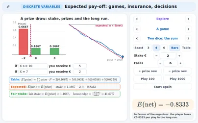
Expected pay-off and the fair stake
Give each outcome its pay-off: the net result N = prize − stake. The expected net result E(N) is what a player gains on average. The game is fair when E(N)=0: the stake equals the expected prize.
Example
A prize draw → €10 with P=0.1, €2 with 0.3, else nothing. The expected prize is 10⋅0.1+2⋅0.3=1.6.A ticket of €2 gives E(N)=1.6−2=−0.4; the fair price is €1.60.
Rule
The organiser’s share and insurance
In the long run the organiser keeps stake − expected prize per ticket, and an insurer needs a premium above the expected claim. For n customers the totals add up: the mean grows with n, the standard deviation only with n.
Example
A claim of €800 has chance 0.005 (1 in 200) → E=800⋅0.005=4. A premium of €6 leaves €2 per customer.10000 customers give €20000; σ≈56.4 each, so about 5640 in total, and the profit stays above 20000−2⋅5640=8720.
Tip
A decision: mean and spread
Compare options by the expected value and by the spread. A higher mean is better only if you can live with the risk; an option with a sure pay-off has standard deviation 0.
Example
A → €20 with P=0.3, else 0 → E=6, σ≈9.2.B → €4 or €9, equally likely → E=6.5, σ=2.5. B has the higher mean and the smaller spread.
Tip
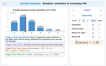
The guess test and a fair penalty
With k choices a guess is right with chance k1. For +1 for a right answer and −m for a wrong one, guessing is fair when k1−kk−1m=0, that is m=k−11.
Example
4 choices, −41 for a wrong answer → E=41−43⋅41=161 per question.Guessing all 20 gives 20⋅161=1.25 marks on average. The fair penalty is 31.
Tip
Stock: unsold items and lost sales
With stock s and demand D: unsold =s−D when D<s, lost sales =D−s when D>s. Find the expected unsold and lost numbers, price them, and choose the stock with the lowest expected cost.
Example
Demand 8,9,10,11,12 with P=0.1,0.2,0.4,0.2,0.1; unsold costs €2, a lost sale €3. For s=10:unsold 2⋅0.1+1⋅0.2=0.4, lost 1⋅0.2+2⋅0.1=0.4, cost 2⋅0.4+3⋅0.4=2. For s=9 the cost is 3.5, for s=11 it is 2.5.
Tip
Warranty: many items together
Each of n independent items fails with chance p and a repair costs c. One item costs pc on average; n items give E=npc and Var=np(1−p)c2, so the spread grows only with n.
Example
n=50, p=0.04, c=€30 → E=50⋅0.04⋅30=60.Var=50⋅0.0384⋅900=1728, σ≈41.6. With 200 items the mean is 240, but σ is only 83.1.
Tip
Which course asks what
Cambridge A level: table, E and Var (Paper 5), aX+b and sums (Paper 6). IB SL: table, E(X), uses; IB HL: variance and linear combinations. AP Statistics: table, mean and SD of a discrete variable. UK GCSE: risk and expected outcome. UK A level: the table only, no mean or variance (Further Maths). Wiskunde A and C vwo → E and σ (school exam); D: also rules for dependent variables. CCSS: S-MD.
Example
Ask which course your class follows, then choose the cards: the table and E(X) for all, Var, aX+b and sums for IB HL, Cambridge Paper 6 and wiskunde D, pay-offs for GCSE and CCSS.
Exercises
A table has x=1,2,3,4 with P=0.15,0.35,0.3,k. Find k. Easy
Show solution
The probabilities add up to 1.
0.15+0.35+0.3+k=1, so 0.8+k=1.
k=0.2
Check → 0.15+0.35+0.3+0.2=1, and 0.2 is between 0 and 1.
x=1,2,3,4 with P=0.1,0.3,0.4,0.2. Find P(X≥3). Easy
Show solution
Add the values in the event → P(X=3)+P(X=4)=0.4+0.2.
Or by the complement → 1−P(X≤2)=1−(0.1+0.3).
P(X≥3)=0.6
Check → both routes give 0.6.
x=0,1,2,3 with P=0.2,0.3,0.3,0.2. Find E(X). Easy
Show solution
Multiply each value by its probability → 0⋅0.2=0, 1⋅0.3=0.3, 2⋅0.3=0.6, 3⋅0.2=0.6.
Add → 0.3+0.6+0.6=1.5.
E(X)=1.5
Check → the table is symmetric about 1.5, so the balance point is 1.5.
A spinner has 4 equal sectors numbered 1,1,2,3. X is the number it shows. Give the table and E(X). Easy
Show solution
Two of the four sectors show 1 → P(X=1)=42=21 and P(X=2)=P(X=3)=41.
E(X)=1⋅21+2⋅41+3⋅41=47.
P=21,41,41 and E(X)=47=1.75
Check → 21+41+41=1, and 1.75 lies between 1 and 3.
E(X)=4 and Var(X)=9. Find E(Y), Var(Y) and σY for Y=2X+5. Easy
Show solution
E(Y)=2⋅4+5=13.
Var(Y)=22⋅9=36; the +5 does not count.
σY=36=6=2⋅3.
E(Y)=13, Var(Y)=36, σY=6
Check → σX=3 and σY=∣2∣⋅3=6.
x=1,2,3,4 with P=0.1,0.2,0.3,0.4. Find F(3) and P(1<X≤3). Easy
Show solution
Add up the probabilities → F(1)=0.1, F(2)=0.1+0.2=0.3, F(3)=0.3+0.3=0.6.
P(1<X≤3)=F(3)−F(1)=0.6−0.1=0.5.
F(3)=0.6 and P(1<X≤3)=0.5
Check → P(X=2)+P(X=3)=0.2+0.3=0.5.
P(X=x)=k(5−x) for x=1,2,3,4. Find k, P(X≤2) and E(X). Medium
Show solution
The weights are 4k,3k,2k,k → 10k=1, so k=0.1.
The table is 0.4,0.3,0.2,0.1, so P(X≤2)=0.4+0.3=0.7.
E(X)=1⋅0.4+2⋅0.3+3⋅0.2+4⋅0.1=2.
k=0.1, P(X≤2)=0.7, E(X)=2
Check → 0.4+0.3+0.2+0.1=1, and the bars fall away to the right, so E(X) lies left of the middle 2.5.
Two fair dice are thrown. X is the larger of the two numbers. Give the table and find E(X). Medium
Show solution
Count the pairs with larger number k → 2k−1 of the 36; 1,3,5,7,9,11.
P(X=k)=362k−1; check 1+3+5+7+9+11=36.
E(X)=361⋅1+2⋅3+3⋅5+4⋅7+5⋅9+6⋅11=36161.
P(X=k)=362k−1 and E(X)=36161≈4.472
Check → 4.47 is above 3.5: the larger of two numbers tends to be high.
x=1,2,4 with P=0.5,0.3,0.2. Find Var(X) by both routes. Medium
Route 2 → E(X2)=0.5+1.2+3.2=4.9 and 4.9−1.92=4.9−3.61=1.29.
Var(X)=1.29, σ≈1.136
Check → the two routes agree, and a variance is never negative.
X is the score of a fair die with 4 faces. Find E(Y), Var(Y) and σY for Y=4−3X. Medium
Show solution
E(X)=41+2+3+4=2.5 and Var(X)=41+4+9+16−2.52=1.25.
E(Y)=4−3⋅2.5=−3.5.
Var(Y)=(−3)2⋅1.25=11.25 and σY=3σX≈3.35.
E(Y)=−3.5, Var(Y)=11.25, σY≈3.35
Check → the variance is positive although a=−3: it is a2=9 times 1.25.
A wheel pays €8 with chance 81, €2 with chance 83 and nothing otherwise. Find the fair stake. A ticket costs €2: what does the organiser expect to gain from 400 plays? Medium
Show solution
Expected prize → 8⋅81+2⋅83=1+43=47. The fair stake equals it.
At a stake of €2 the organiser gains 2−47=41 per play.
For 400 plays → 400⋅41=100.
Fair stake €1.75; expected gain €100
Check → the player expects E(N)=1.75−2=−0.25 per play, so 400⋅0.25=100 in all.
A die has σ≈1.71. How big is the typical gap between the mean of n throws and 3.5 for n=100 and for n=400? Medium
Show solution
The typical gap is about σ/n.
n=100 → 101.71≈0.17.
n=400 → 201.71≈0.085, half as big.
About 0.17 for n=100 and 0.085 for n=400
Check → four times as many throws halve the gap; 4=2.
Two fair dice are thrown and X is the sum. Find P(X≥10), E(X) and Var(X). Hard
Show solution
Count the pairs → the sums 10,11,12 come in 3,2,1 ways, so P(X≥10)=366=61.
Each die has E=3.5 and Var=1235, and the dice are independent.
E(X)=3.5+3.5=7 and Var(X)=1235+1235=635.
P(X≥10)=61, E(X)=7, Var(X)=635
Check → the table of the sum gives E(X2)=6329 and 6329−49=635.
x=1,2,3 with P=0.61,k,k2. Find k and E(X). Hard
Show solution
The sum is 1 → 0.61+k+k2=1, so k2+k−0.39=0.
(k−0.3)(k+1.3)=0, so k=0.3 or k=−1.3. A probability cannot be negative, so k=0.3.
The table is 0.61,0.3,0.09 and E(X)=0.61+0.6+0.27=1.48.
k=0.3 and E(X)=1.48
Check → 0.61+0.3+0.09=1 and −1.3 would give a probability −1.3.
X and Y have E(X)=3, Var(X)=2, E(Y)=5, Var(Y)=4. Let W=2X−3Y+1. Find E(W) and Var(W) when X and Y are independent, and when Cov(X,Y)=0.5. Hard
Show solution
E(W)=2⋅3−3⋅5+1=−8 in both cases.
Independent → Var(W)=22⋅2+(−3)2⋅4=8+36=44, so σW=44=211≈6.63.
Check → the cross term is negative because 2 and −3 have opposite signs, so a positive covariance lowers the variance.
A player pays €2 for a wheel that pays €8 (chance 81), €2 (83) or nothing, so N=6,0 or −2. Find E(N) and Var(N), and the mean and SD of the total of 900 plays. Hard
Show solution
E(N)=6⋅81+0−2⋅21=−41.
E(N2)=36⋅81+4⋅21=213, so Var(N)=213−161=16103.
900 plays → mean −225, σ=900⋅16103≈76.1.
E(N)=−0.25, Var(N)=6.4375; the total has mean −225 and σ≈76.1
Check → the organiser gains 225±2⋅76.1, about 73 to 377, above 0.
Demand is 8 to 12 with P=0.1,0.2,0.4,0.2,0.1. Unsold costs €1, a lost sale €4. Which stock s out of 10,11,12 costs least? Hard
Show solution
s=10 → unsold 0.4, lost 0.4, cost 1⋅0.4+4⋅0.4=2.
s=11 → unsold 1.1, lost 0.1, cost 1.1+4⋅0.1=1.5.
s=12 → unsold 2, lost 0, cost 2.
s=11 with an expected cost of €1.5
Check → a lost sale costs more than an unsold item, so the best stock is above the most likely demand 10.
X and Y are each 0 or 1 with p00=p11=0.3 and p01=p10=0.2. Find Cov(X,Y) and Var(X+Y), and check with the table of X+Y. Hard
Show solution
P(X=1)=0.2+0.3=0.5, so E(X)=E(Y)=0.5 and Var(X)=Var(Y)=0.25.
E(XY)=1⋅1⋅0.3=0.3, so Cov=0.3−0.25=0.05.
Var(X+Y)=0.25+0.25+2⋅0.05=0.6.
Cov(X,Y)=0.05 and Var(X+Y)=0.6
Check → X+Y is 0,1,2 with 0.3,0.4,0.3; E=1, E(X2)=0.4+1.2=1.6 and 1.6−1=0.6.
Interactive applications for this topic
Free applications open with a free student account. Teachers can use all applications in a live lesson.